
Filtering in Pandas: Learn loc, iloc, isin(), and between()
Filtering in Pandas is a key part of analyzing data. This approach makes it much easier to find your way around and understand your data by letting you choose specific rows or columns based on certain conditions.
You might need to get certain information from a DataFrame in Python instead of using the whole thing. This is called filtering, and it lets you rapidly discover the rows or columns that are important to you.
Pandas makes filtering easier by giving you two options: loc and iloc.
What is Filtering in Pandas?
Filtering is the process of picking out data that meets a certain need.
For instance, finding customers over 30 or sales from a certain group.
Filtering is useful:
Pay attention to data that matters
Before analyzing, clean up the datasets.
Make results faster and clearer
Setting Up the Dataset
Download Sample Dataset: retail_sales_dataset
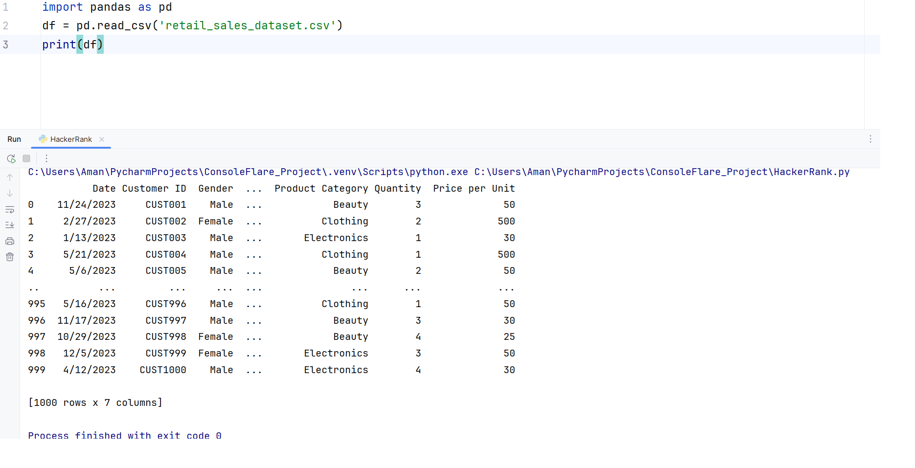
We’ll use a sample file called retail_sales_dataset.csv.
Python
Output:
1. Filtering with iloc—Based on where the index is
Index location is what iloc stands for.
It uses the numeric index to filter rows or columns.
Example 1: Get one row
Python
displays information from row one (index 0).
Example 2: Get multiple rows in a Data Frame
You should simply specify a list of indexes in iloc to obtain multiple rows in the dataframe.
displays rows that have the indexes 0, 3, and 5.
Output
|    | Customer ID | Gender | Age | Product Category | Quantity | Price per Unit |
| -: | ----------- | ------ | --: | ---------------- | -------: | -------------: |
|  0 | CUST001     | Male   |  34 | Beauty           |        3 |             50 |
|  3 | CUST004     | Male   |  37 | Clothing         |        1 |            500 |
|  5 | CUST006     | Female |  45 | Beauty           |        1 |             30 |
Example 3: Slice rows
You should simply use index slicing, as we did in Python, to slice multiple rows in a dataframe.
Gives rows from index 2 to 4.
Output
|     | Customer ID | Gender | Age | Product Category | Quantity | Price per Unit |
| --: | ----------- | ------ | --: | ---------------- | -------: | -------------: |
|   0 | CUST001     | Male   |  34 | Beauty           |        3 |             50 |
|   1 | CUST002     | Female |  26 | Clothing         |        2 |            500 |
|   2 | CUST003     | Male   |  50 | Electronics      |        1 |             30 |
|   3 | CUST004     | Male   |  37 | Clothing         |        1 |            500 |
|   4 | CUST005     | Male   |  30 | Beauty           |        2 |             50 |
| ... | ...         | ...    | ... | ...              |      ... |            ... |
| 995 | CUST996     | Male   |  62 | Clothing         |        1 |             50 |
| 996 | CUST997     | Male   |  52 | Beauty           |        3 |             30 |
| 997 | CUST998     | Female |  23 | Beauty           |        4 |             25 |
| 998 | CUST999     | Female |  36 | Electronics      |        3 |             50 |
| 999 | CUST1000    | Male   |  47 | Electronics      |        4 |             30 |
Example 4: Get a single value
A single value has two indexes. To get a single value, you need to specify the row and column index.
provides the value found in the first column and row.
Example 5: Get random rows and columns
To get random rows and random columns from dataframe, you should specify the list of rows and list of columns.
Python
Output
|    | Customer ID | Age | Quantity |
| -: | ----------- | --: | -------: |
|  0 | CUST001     |  34 |        3 |
|  3 | CUST004     |  37 |        1 |
|  5 | CUST006     |  45 |        1 |
Example 6: Slice rows and columns
You can use slicing of rows and columns in dataframe.
displays rows 0–2 and columns 2–3 (Product Category, Age).
Output
|    | Age | Product Category |
| -: | --: | ---------------- |
|  0 |  34 | Beauty           |
|  1 |  26 | Clothing         |
|  2 |  50 | Electronics      |
Example 7: Get a full column
You can get single column by slicing index of all rows and single column.
df.iloc[:, 1]2. Using loc for filtering based on conditions
When filtering based on values rather than index numbers, loc is utilized.
Logical conditions are applicable to any column.
Syntax:
df.loc[condition]Example 1: Gender = Male
df.loc[df['Gender'] == 'Male']Output
|    | Customer ID | Gender | Age | Product Category | Quantity | Price per Unit |
| -: | ----------- | ------ | --: | ---------------- | -------: | -------------: |
|  0 | CUST001     | Male   |  34 | Beauty           |        3 |             50 |
|  2 | CUST003     | Male   |  50 | Electronics      |        1 |             30 |
|  3 | CUST004     | Male   |  37 | Clothing         |        1 |            500 |
|  4 | CUST005     | Male   |  30 | Beauty           |        2 |             50 |
|  6 | CUST007     | Male   |  46 | Clothing         |        2 |             25 |
Example 2: Age > 50
df.loc[df['Age'] > 50]Output
|    | Customer ID | Gender | Age | Product Category | Quantity | Price per Unit |
| -: | ----------- | ------ | --: | ---------------- | -------: | -------------: |
|  8 | CUST009     | Male   |  63 | Electronics      |        2 |            300 |
|  9 | CUST010     | Female |  52 | Clothing         |        4 |             50 |
| 13 | CUST014     | Male   |  64 | Clothing         |        4 |             30 |
| 18 | CUST019     | Female |  62 | Clothing         |        2 |             25 |
| 24 | CUST025     | Female |  64 | Beauty           |        1 |             50 |
Example 3: Product Category != Electronics
Multiple Conditions in Filtering
Logical operators can be used to combine several conditions:
| Symbol | Meaning | Example |
|---|---|---|
& |
and | (df['Gender']=='Male') & (df['Age']>50) |
| ` | ` | or |
!= |
not equal | df['Category'] != 'Electronics' |
~ |
NOT | ~(df['Gender']=='Male') |
Example 1: Male and Age > 50
Output
|     | Customer ID | Gender | Age | Product Category | Quantity | Price per Unit |
| --: | ----------- | ------ | --: | ---------------- | -------: | -------------: |
|   8 | CUST009     | Male   |  63 | Electronics      |        2 |            300 |
|  13 | CUST014     | Male   |  64 | Clothing         |        4 |             30 |
|  35 | CUST036     | Male   |  52 | Beauty           |        3 |            300 |
|  47 | CUST048     | Male   |  54 | Electronics      |        3 |            300 |
|  58 | CUST059     | Male   |  62 | Clothing         |        1 |             50 |
| ... | ...         | ...    | ... | ...              |      ... |            ... |
| 969 | CUST970     | Male   |  59 | Electronics      |        4 |            500 |
| 972 | CUST973     | Male   |  60 | Clothing         |        1 |             50 |
| 983 | CUST984     | Male   |  56 | Clothing         |        1 |            500 |
| 995 | CUST996     | Male   |  62 | Clothing         |        1 |             50 |
| 996 | CUST997     | Male   |  52 | Beauty           |        3 |             30 |
Example 2: Age between 20 and 30
Output
|    | Customer ID | Gender | Age | Product Category | Quantity | Price per Unit |
| -: | ----------- | ------ | --: | ---------------- | -------: | -------------: |
|  1 | CUST002     | Female |  26 | Clothing         |        2 |            500 |
| 10 | CUST011     | Male   |  23 | Clothing         |        2 |             50 |
| 12 | CUST013     | Male   |  22 | Electronics      |        3 |            500 |
| 16 | CUST017     | Female |  27 | Clothing         |        4 |             25 |
| 19 | CUST020     | Male   |  22 | Clothing         |        3 |            300 |
Example 3: Category Clothing or Electronics
Output
|    | Customer ID | Gender | Age | Product Category | Quantity | Price per Unit |
| -: | ----------- | ------ | --: | ---------------- | -------: | -------------: |
|  1 | CUST002     | Female |  26 | Clothing         |        2 |            500 |
|  2 | CUST003     | Male   |  50 | Electronics      |        1 |             30 |
|  3 | CUST004     | Male   |  37 | Clothing         |        1 |            500 |
|  6 | CUST007     | Male   |  46 | Clothing         |        2 |             25 |
|  7 | CUST008     | Male   |  30 | Electronics      |        4 |             25 |
Example 4: Category not Electronics
Output
|    | Customer ID | Gender | Age | Product Category | Quantity | Price per Unit |
| -: | ----------- | ------ | --: | ---------------- | -------: | -------------: |
|  0 | CUST001     | Male   |  34 | Beauty           |        3 |             50 |
|  1 | CUST002     | Female |  26 | Clothing         |        2 |            500 |
|  3 | CUST004     | Male   |  37 | Clothing         |        1 |            500 |
|  4 | CUST005     | Male   |  30 | Beauty           |        2 |             50 |
|  5 | CUST006     | Female |  45 | Beauty           |        1 |             30 |
Example 5: Not Male and not Electronics
Output
|    | Customer ID | Gender | Age | Product Category | Quantity | Price per Unit |
| -: | ----------- | ------ | --: | ---------------- | -------: | -------------: |
|  0 | CUST001     | Male   |  34 | Beauty           |        3 |             50 |
|  1 | CUST002     | Female |  26 | Clothing         |        2 |            500 |
|  3 | CUST004     | Male   |  37 | Clothing         |        1 |            500 |
|  4 | CUST005     | Male   |  30 | Beauty           |        2 |             50 |
|  5 | CUST006     | Female |  45 | Beauty           |        1 |             30 |
Useful Filtering Functions
1. isin() – Check Multiple Values
Ouput
|    | Customer ID | Gender | Age | Product Category | Quantity | Price per Unit |
| -: | ----------- | ------ | --: | ---------------- | -------: | -------------: |
|  1 | CUST002     | Female |  26 | Clothing         |        2 |            500 |
|  2 | CUST003     | Male   |  50 | Electronics      |        1 |             30 |
|  3 | CUST004     | Male   |  37 | Clothing         |        1 |            500 |
|  6 | CUST007     | Male   |  46 | Clothing         |        2 |             25 |
|  7 | CUST008     | Male   |  30 | Electronics      |        4 |             25 |
2. between() – Filter by Range
Output
|     | Customer ID | Gender | Age | Product Category | Quantity | Price per Unit |
| --: | ----------- | ------ | --: | ---------------- | -------: | -------------: |
|   1 | CUST002     | Female |  26 | Clothing         |        2 |            500 |
|   4 | CUST005     | Male   |  30 | Beauty           |        2 |             50 |
|   7 | CUST008     | Male   |  30 | Electronics      |        4 |             25 |
|  10 | CUST011     | Male   |  23 | Clothing         |        2 |             50 |
|  12 | CUST013     | Male   |  22 | Electronics      |        3 |            500 |
| ... | ...         | ...    | ... | ...              |      ... |            ... |
| 970 | CUST971     | Female |  27 | Electronics      |        4 |             50 |
| 980 | CUST981     | Female |  30 | Electronics      |        2 |             30 |
| 982 | CUST983     | Female |  29 | Clothing         |        1 |            300 |
| 986 | CUST987     | Female |  30 | Clothing         |        3 |            300 |
| 997 | CUST998     | Female |  23 | Beauty           |        4 |             25 |
3. reset_index() – Clean Up After Filtering
Filtering causes the indexes to lose their serial order. The dataframe’s index can be reset using reset_index().
- The index is reset by the reset_index() function.
reset_index(drop=True) removes the previous index from the dataframe and resets the index instead.
Output
|     | Customer ID | Gender | Age | Product Category | Quantity | Price per Unit |
| --: | ----------- | ------ | --: | ---------------- | -------: | -------------: |
|   0 | CUST002     | Female |  26 | Clothing         |        2 |            500 |
|   1 | CUST005     | Male   |  30 | Beauty           |        2 |             50 |
|   2 | CUST008     | Male   |  30 | Electronics      |        4 |             25 |
|   3 | CUST011     | Male   |  23 | Clothing         |        2 |             50 |
|   4 | CUST013     | Male   |  22 | Electronics      |        3 |            500 |
| ... | ...         | ...    | ... | ...              |      ... |            ... |
| 226 | CUST971     | Female |  27 | Electronics      |        4 |             50 |
| 227 | CUST981     | Female |  30 | Electronics      |        2 |             30 |
| 228 | CUST983     | Female |  29 | Clothing         |        1 |            300 |
| 229 | CUST987     | Female |  30 | Clothing         |        3 |            300 |
| 230 | CUST998     | Female |  23 | Beauty           |        4 |             25 |
Update records
Let’s say you wish to raise Beauty’s price from 50 to 100. The value can be updated using the.loc property.
Python
df.loc[df['Product Category'] == 'Beauty', 'Price per Unit'] = 100
df.head()
Output
| Customer ID | Gender | Age | Product Category | Quantity | Price per Unit |
|---|---|---|---|---|---|
| CUST001 | Male | 34 | Beauty | 3 | 50 |
| CUST002 | Female | 26 | Clothing | 2 | 500 |
| CUST003 | Male | 50 | Electronics | 1 | 30 |
| CUST004 | Female | 22 | Beauty | 5 | 20 |
| CUST005 | Male | 60 | Clothing | 2 | 700 |
Additionally, you can use more than one condition. Let’s say you wish to raise the price of a male clothing product from 500 to 1,000.
Python
df.loc[(df['Gender'] == 'Male') & (df['Product Category'] == 'Clothing'), 'Price per Unit'] = 1000
df.head()
Output
| Customer ID | Gender | Age | Product Category | Quantity | Price per Unit |
|---|---|---|---|---|---|
| CUST001 | Male | 34 | Beauty | 3 | 100 |
| CUST002 | Female | 26 | Clothing | 2 | 500 |
| CUST003 | Male | 50 | Electronics | 1 | 30 |
| CUST004 | Female | 22 | Beauty | 5 | 1000 |
| CUST005 | Male | 60 | Clothing | 2 | 100 |
Common Mistakes
Missing parentheses in multiple conditions
df['Age'] > 20 & df['Age'] < 30(df['Age'] > 20) & (df['Age'] < 30)
Using and / or instead of & / |
Forgetting df.loc[] before conditions
Related Post:
Load Data in Pandas – A Complete Beginner’s Guide to Data Import
Summary
For index-based filtering, utilize iloc. Utilize loc for filtering based on conditions.Employ logical operators to combine filters.Employ helper functions such as between() and isin().Reset the index after filtering every time.Filtering makes it easier to swiftly extract the appropriate data. You can handle the majority of real-world datasets with ease once you comprehend how loc and iloc function.
For more such content and regular updates, follow us on Facebook, Instagram, and LinkedIn
Conclusion:
The fusion of data science in the finance sector is not just a technological evolution but also a fundamental shift in the way the financial industry operates. From predictive analytics to personalized financial services, the applications of data science are reshaping traditional practices and opening up new possibilities. As we all move forward, the synergy between finance and data science will continue to evolve, creating a more robust, efficient, and resilient financial ecosystem. In this data-driven era, those who embrace the power of data science will be at the forefront of innovations and success in the world of finance. Want to know what else can be done by Data Science? If you wish to learn more about data science or want to advance your career in the data science field, feel free to join our free workshop on Masters in Data Science with PowerBI, where you will get to know how exactly the data science field works and why companies are ready to pay handsome salaries in this field. In this workshop, you will get to know each tool and technology from scratch, which will make you skillfully eligible for any data science profile .To join this workshop, register yourself on ConsoleFlare, and we will call you back.
Thinking, Why Console Flare?
Recently, ConsoleFlare has been recognized as one of the Top 10 Most Promising Data Science Training Institutes of 2023.
Console Flare offers the opportunity to learn Data Science in Hindi, just like how you speak daily.
Console Flare believes in the idea of “What to learn and what not to learn,” and this can be seen in their curriculum structure. They have designed their program based on what you need to learn for data science and nothing else.
Want more reasons?
Register yourself on ConsoleFlare, and we will call you back.
Log in or sign up to view
See posts, photos, and more on Facebook.